
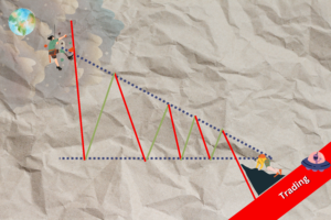
The second triangle: the Descending Triangle
Read More


5 Common Mistakes Beginner Traders Make
Things to avoid when you’re just starting to trade
Read More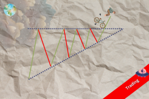
Trading Dow Pattern the Triangle Pattern (Part 1)
The first triangle: the Ascending Triangle
Read More
Funds: Equity Funds (Part 3)
How to choose between equity funds based on companies’ earnings...
Read More